Fractals, by definition, have patterns that occur on many scales. This scaling can be in either the time or spatial dimensions. Because patterns repeat, and those patterns occur with different frequencies, due to their scale, they ought to be amenable to analysis by Fourier transforms.
Fourier transforms are an efficient technique for decomposing a signal in the time or spatial domain into the frequency domain. So, for example, if a recording of music were put through a Fourier transform, the result would be the musical notes that constituted it, as well as all the harmonics of the instruments that played it. The output loses the time domain; instead, it has the amplitudes of all the frequencies that composed it, as well as the phases of the sine-waves at those frequencies. The astonishing thing about this technique is that it is fully reversible and the original music can be reconstructed from just the knowing the frequencies and phases using the inverse transform.
In the digital domain, the Fast Fourier Transform (FFT) is king. It is a highly efficient way of performing frequency analysis of digital information. It works with discrete samples of the waveforms. FFTs can be performed in any number of dimensions. One dimensional FFTs are useful for analysis of things like sound. Two-dimensional FFTs are useful for analysis of images. Three-dimensional FFTs are useful for analysis of videos (2 dimensions of space and one of time) or 3d models.
Previously in the Speed Camera project, FFTs were used to extract the speed of moving vehicles from the Doppler-shifted frequencies created when radar signals bounce off moving objects.
Surprisingly, there is very little information available on the analysis of fractals in the frequency domain; what can be found is behind the paywalls of academic journals and mostly relating to the study of cardiology; hence this work.
A basic set of tools were composed using the JTransforms library to perform the transforms and render images. If there is interest, these can be uploaded to GitHub.
Mandelbrot Set
The Mandelbrot set is the archetypal fractal. It produces beauty from the simplest of mathematical origins. The Mandelbrot set has so many fascinating corners that it is easy to get lost in time exploring it. The patterns it contains subtly morph in scale and shape around its edge.
The following diagram summarises the author’s explorations of the Mandelbrot set. A simple rendering of the fractal in the region of -2 to +2 in the real and imaginary dimensions was generated. The Mandelbrot set requires complex numbers.) The rendering is shown in the top left corner of Figure 1. Below it is shown a zoomed-in fragment of the detail, showing the self-similarity. Below that, in the lower left corner of Figure 1, is the same Mandelbrot set transformed from polar to rectangular coordinates. This transforms the image such that rotation around the origin becomes distance across the image (the x-axis), and distance from the centre the y-axis.
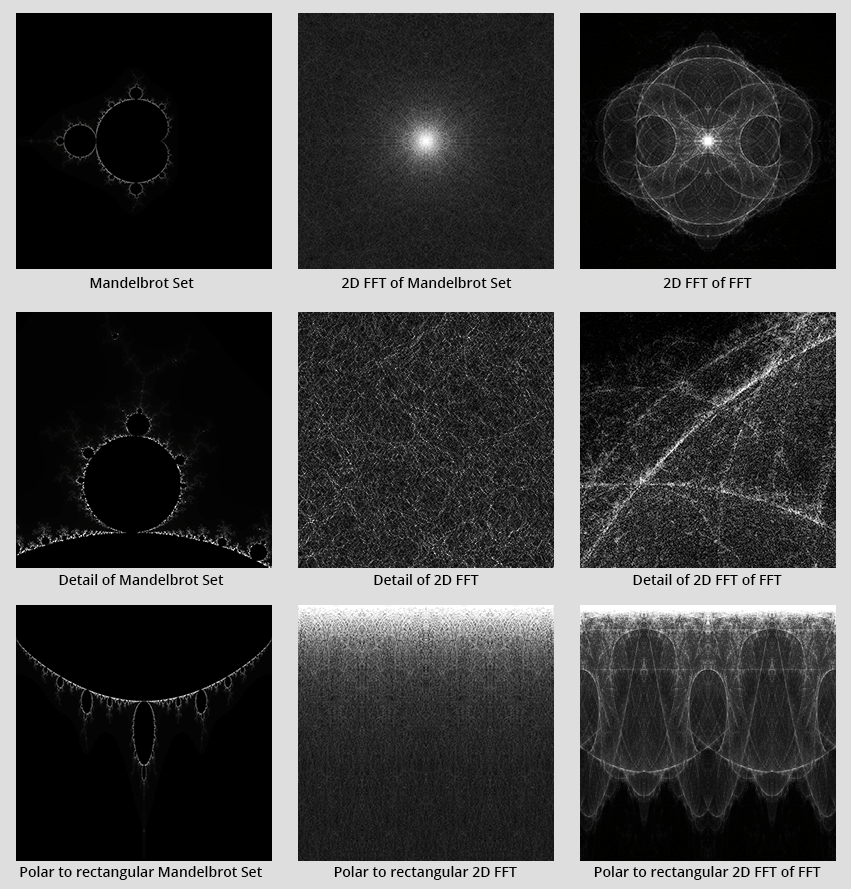 Figure 1: Frequency analysis of the Mandelbrot set
The mechanism of the FFT transform requires some explanation: The reality of the implementation is that it takes complex numbers in, and gives complex numbers out. The 2-dimensional transform we are using here requires a 2-dimensional matrix of complex numbers. We assign the pixel brightness to the real part and set the imaginary part to zero. The transform generates a result in a 2-dimensional matrix of the same size, but now each point in the matrix relates to frequencies rather than position. The exact mapping is a little difficult to understand so we will not get into it in too much detail in this post. For each point in the output matrix, we can extract both the magnitude of the complex number and the phase. In the plots, in Figure 1 we only show the magnitude. The phase component contains valuable information to reconstruct the input signal, but when visualised looks rather meaningless. (See Figure 2 for an example.)
The magnitude component of the FFT transform on the Mandelbrot set shows some unexpected and remarkable detail. It appears as layers of fine threads that look reminiscent of the renderings of dark matter distribution. This structure is all the more surprising after looking at other fractals - see Figure 4. Natural fractals appear to contain almost white-noise like, uniform, frequency distributions, whereas simpler artificial fractals contain very geometric patterns in the spectra.
The resultant image from performing a second FFT on the image generated from the first FFT was extraordinary - with a structure less perfect than the original Mandelbrot, but no less elegant, it has delicate intersections of complex curves exposed. This could be the x-ray of an alien creature. The author is unsure of the mathematical meaning of this second order FFT transform, but It could be thought of as the frequency distribution of the frequency distribution. This is somewhat similar to the repeated differentiation in calculus whereby differentiation of position gives velocity, and differentiation of velocity results determines acceleration.
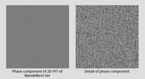 Figure 2: Phase Component
After finding thought-provoking detail in this second order FFT, the author decided to delve deeper. Unfortunately, there appears to be no additional interest lower down as can be seen in Figure 3. The spectra appears to fall into almost uniform noise.
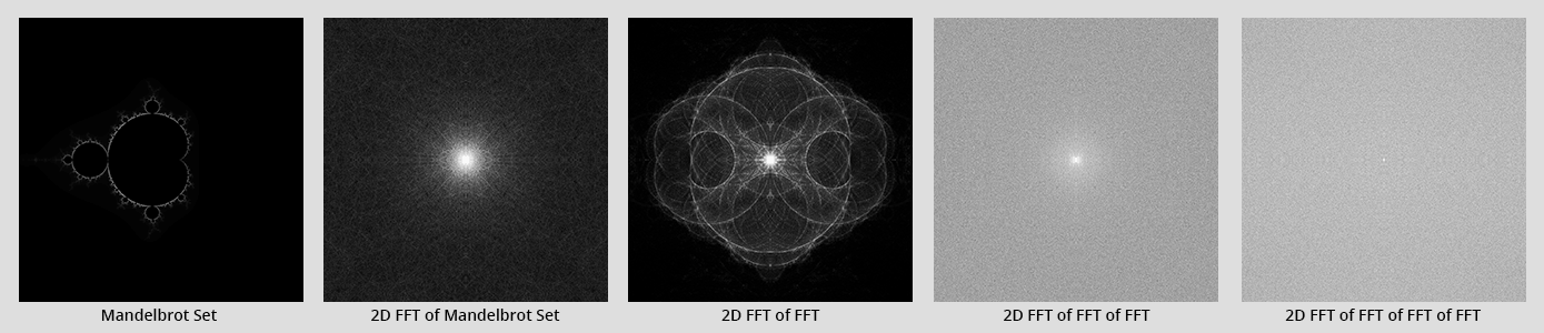 Figure 3: Continued analysis of the Mandelbrot set
Other Fractals
Other fractals have been analysed with a similar technique. Figure 4 presents the results. It is worth noting that the artificial fractals of the Julia set, Menger sponge and Hilbert curve all show self-similar structure on the second order FFTs. Natural fractals taken from the branch structure of a deciduous tree, and its leaf structure, are less impressive.
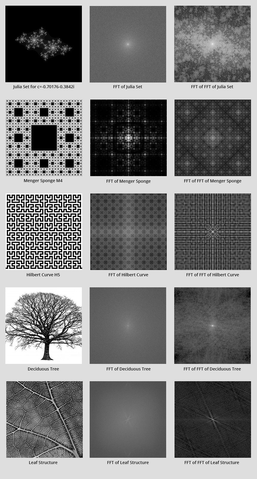 Figure 4: Frequency analysis of other fractals