This paper offers an analysis of the application of NetKernel and Resource oriented computing to the well known Travelling Salesman Problem (TSP).
This discussion ignores the many approximate approaches to solving this problem which are necessary for real-world problems of any significant complexity. The aim, however, is to show how ROC can automatically optimise a solution which it knows nothing about other than empirical data collected during execution.
The algorithm structures the problem into sub-problems many of which overlap with each other - this occurrence is called overlapping subproblems. This decomposition is often used in dynamic programming approaches.
Dynamic programming has the ability to change the computational complexity of the TSP from O(n!) to O(2n). This leads to a significant improvement in execution time for larger problems. The trade-off however is that additional storage space (memory) must be allocated. Dynamic programming achieves this by storing and retrieving sub-problems which it has previously encountered. In the case of the TSP this space requirement grows exponentially with the size of the problem.
NetKernel uses a computation cache which has a similar effect to employing dynamic programming to a problem. For more details of works of this cache see my previous post. However this caching operates differently to dynamic programming in two key ways:
- Automatic optimisation - dynamic programming requires specific instrumentation of the algorithm to store and retrieve sub-problems. The code to do this is specific to the algorithm and only makes sense when the problem is very well defined and the benefits understood. I.e. it works well for specific algorithms but not to general purpose business systems even when they have massive quantities of overlapping subproblems.
- Managing space - dynamic programming usually requires the allocation and deallocation of storage tied to the execution of the algorithm. We already mentioned that TSP requires exponential space requirements. It requires this space for the duration of execution. What happens if we don’t have that much space? Can we gain benefit from dynamic programming? - NO! Another problem is that all stored sub-problems are identified relative to the context of the algorithm execution - there is no memory of repeated sub-problems in the larger timescale.
For more details of the close relationship between ROC caching and dynamic programming see my previous post.
Scenario 1 - Study the effects of cache size on execution performance
In this scenario we solve a 13 vertex travelling salesman problem. We generate a random asymmetric graph with 50 uni-directional edges evenly distributed between the vertices.

Each iteration uses the same seeded graph but we vary the size of the NetKernel cache. We vary the size from 20000 which holds all-subproblems down to 5000 which is too small to hold any reasonable fraction of the sub-problems. Between each iteration we clear the cache.
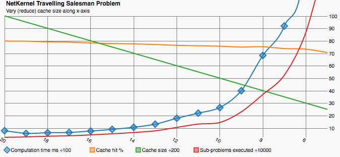
We can plainly see how computation time increases as the cache size decreases. There is a proportional increase in the number of sub-problems executed which show additional computation happening where results could not be retrieved from cache. Clearly we can choose a trade-off between time and space it’s not an all or nothing affair.
It is somewhat surprising that the cache hit rate remains so high - only dropping from 80% to 71% across the range. I believe this shows two things - firstly that even a small cache can lead to large benefits and larger caches lead to diminishing returns. I have not analysed the distribution of sub-problem re-use by TSP. However often requests follow normal or power-set distributions.
The second thing that the steady cache hit rate shows is an artefact of the cache implementation. The execution time is so short and the cache size is only maintained by culling once the maximum size is reached. This leads to us operating with an average actual cache size significantly larger than the headline figure.
| Cache size | Compute Time (ms) | Cached sub-problems | Cache Hit % | sub-problems executed |
|---|---|---|---|---|
| 20050 | 810 | 16155 | 0.80 | 279545 |
| 19050 | 596 | 18402 | 0.80 | 310598 |
| 18050 | 645 | 17272 | 0.79 | 369828 |
| 17050 | 669 | 15374 | 0.79 | 402350 |
| 16050 | 781 | 12137 | 0.78 | 474269 |
| 15050 | 918 | 14027 | 0.78 | 563425 |
| 14050 | 1086 | 13675 | 0.78 | 663750 |
| 13050 | 1330 | 9236 | 0.77 | 797041 |
| 12050 | 1806 | 9632 | 0.77 | 1073797 |
| 11050 | 2220 | 7803 | 0.76 | 1341789 |
| 10050 | 2663 | 7262 | 0.76 | 1465122 |
| 9050 | 4016 | 8380 | 0.75 | 2320985 |
| 8050 | 6848 | 7905 | 0.75 | 3713247 |
| 7050 | 9212 | 6207 | 0.74 | 5261161 |
| 6050 | 15633 | 3567 | 0.74 | 8689142 |
| 5050 | 54834 | 4430 | 0.71 | 14962837 |
Table 1 : Raw data for scenario 1
Scenario 2 - Effect of problem complexity
In this scenario we study the effects of varying the problem size on the computational complexity. We generate a series a graphs starting with 4 vertices and increase one vertex at a time up to 15 vertices. We ensure we have a large enough cache size for all available sub-problems.
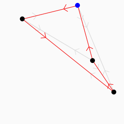 4 vertices
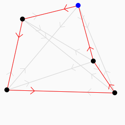 5 vertices
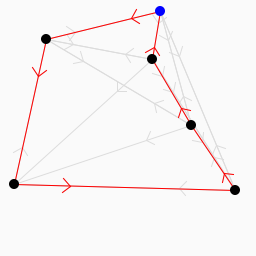 6 vertices
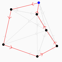 7 vertices
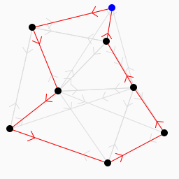 8 vertices
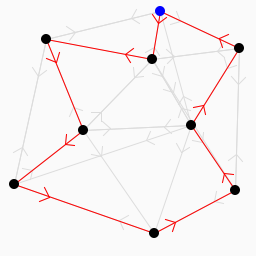 9 vertices
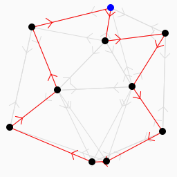 10 vertices
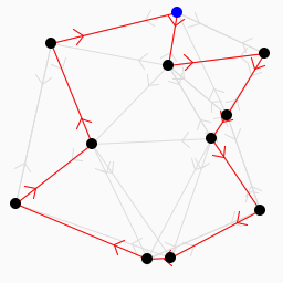 11 vertices
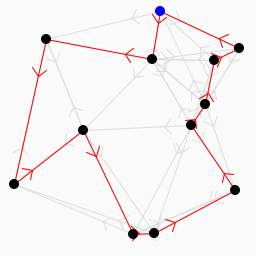 12 vertices
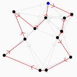 13 vertices
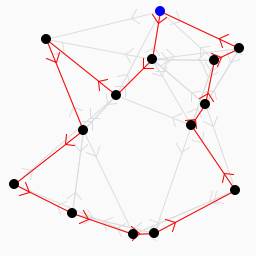 14 vertices
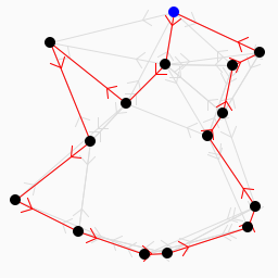 15 vertices
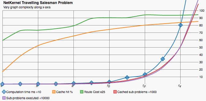
There are a number of interesting observations from this chart. Firstly we see how there is very little cache benefit when the problem size is small. The proportion of overlapping sub-problems increases as the problem size grows.
Computation time, sub-problems executed and cached sub-problems all increase exponentially with the problem size as expected.
The route cost increases as the problem size grows.
| Iteration | Compute Time (ms) | Cached sub-problems | Cache Hit % | sub-problems executed | Route cost |
|---|---|---|---|---|---|
| 4 | 1 | 13 | 0.166 | 5 | 2.364 |
| 5 | 2 | 33 | 0.380 | 41 | 2.900 |
| 6 | 2 | 81 | 0.522 | 177 | 2.928 |
| 7 | 3 | 193 | 0.596 | 638 | 3.008 |
| 8 | 10 | 447 | 0.653 | 2016 | 3.165 |
| 9 | 18 | 1016 | 0.708 | 5260 | 3.563 |
| 10 | 29 | 2281 | 0.742 | 15130 | 3.605 |
| 11 | 90 | 5049 | 0.772 | 39476 | 3.605 |
| 12 | 131 | 11077 | 0.800 | 97332 | 3.757 |
| 13 | 342 | 24082 | 0.818 | 225159 | 3.739 |
| 14 | 801 | 51074 | 0.836 | 515013 | 3.740 |
| 15 | 2055 | 108864 | 0.849 | 1152632 | 3.766 |
Table 2 : Raw data for scenario 2
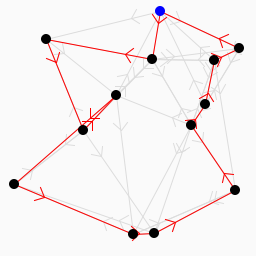
Scenario 3 - Incremental changes to problem
In scenario 3 I want to see how the travelling sales man adapts to incremental changes to the graph. My hypothesis was that we should still see a significant sub-problem overlap when a significant proportion of the problem remains unchanged. This is an attempt to simulate a real world scenario that any traditional optimisation to TSP would miss.
We iterate 20 times from a starting graph of 13 vertices and 50 evenly distributed edges connecting to the closest vertices. On each iteration we take one of the vertices and move it to a new location hence altering the cost of all edges in and out of that vertex.
 Iteration 1
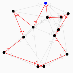 Iteration 2
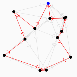 Iteration 3
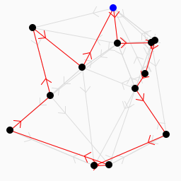 Iteration 4
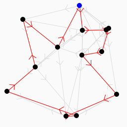 Iteration 5
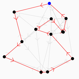 Iteration 6
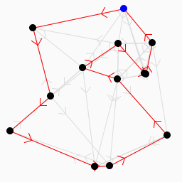 Iteration 7
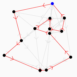 Iteration 8
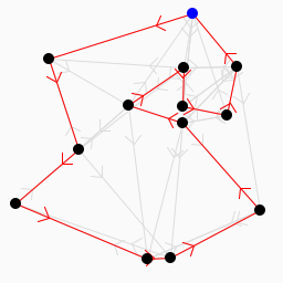 Iteration 9
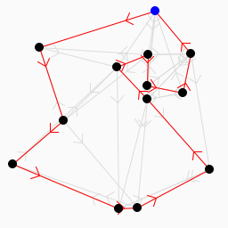 Iteration 10
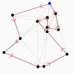 Iteration 11
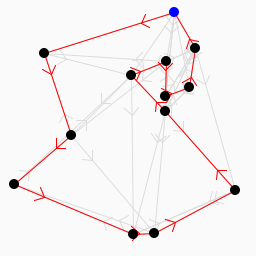 Iteration 12
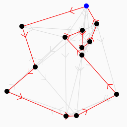 Iteration 13
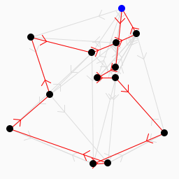 Iteration 14
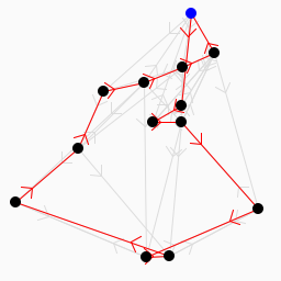 Iteration 15
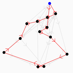 Iteration 16
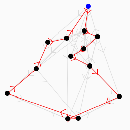 Iteration 17
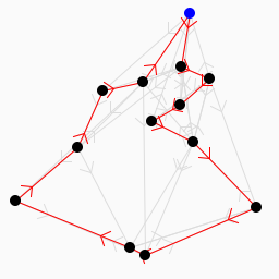 Iteration 18
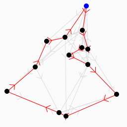 Iteration 19
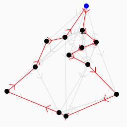 Iteration 20
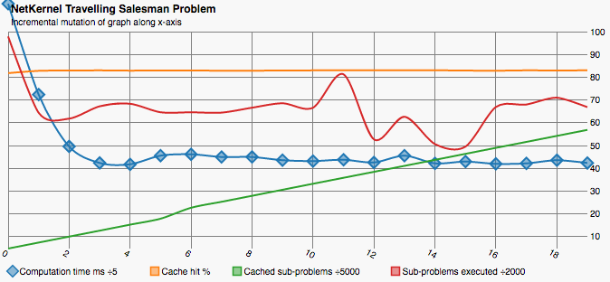
We see that the initial execution has a cost more than double of all subsequent iterations. This shows that a significant saving in computational effort. More importantly this confirms the hypothesis that the NetKernel cache can lead to optimisations not possible with traditional dynamic programming techniques.
Interestingly the ratio of sub-problems executed between first and subsequent iterations is lower than the ratio of computation time. This exposes the fact that cache hits result in saved computation of sub-problem and recursively all sub-sub-problems.
| Iteration | Compute Time (ms) | Cached sub-problems | Cache Hit % | sub-problems executed | Route cost |
|---|---|---|---|---|---|
| 0 | 561 | 24177 | 0.82 | 195789 | 4.007 |
| 1 | 362 | 37317 | 0.83 | 128828 | 4.010 |
| 2 | 248 | 50390 | 0.83 | 123652 | 3.852 |
| 3 | 212 | 63389 | 0.83 | 134469 | 3.806 |
| 4 | 209 | 76608 | 0.83 | 136697 | 3.985 |
| 5 | 228 | 89681 | 0.83 | 129243 | 3.940 |
| 6 | 231 | 113675 | 0.83 | 129243 | 3.953 |
| 7 | 225 | 126748 | 0.83 | 128941 | 4.0269 |
| 8 | 225 | 139868 | 0.83 | 133259 | 3.991 |
| 9 | 218 | 153132 | 0.83 | 137159 | 3.885 |
| 10 | 216 | 166300 | 0.83 | 133226 | 3.847 |
| 11 | 219 | 179392 | 0.83 | 162557 | 3.708 |
| 12 | 213 | 192484 | 0.83 | 105417 | 3.682 |
| 13 | 228 | 205576 | 0.83 | 125327 | 3.765 |
| 14 | 211 | 218696 | 0.83 | 101329 | 3.422 |
| 15 | 215 | 231915 | 0.83 | 99098 | 3.398 |
| 16 | 210 | 245083 | 0.83 | 133888 | 3.375 |
| 17 | 211 | 258139 | 0.83 | 136064 | 3.208 |
| 18 | 218 | 271307 | 0.83 | 142058 | 3.159 |
| 19 | 212 | 284475 | 0.83 | 133746 | 3.220 |
Table 3 : Raw data for scenario 3
Experimental Setup
A fully working NetKernel module with all source code is available. Please contact me for further details.
Conclusions
The paper shows the NetKernel cache shares the compute time optimisations that dynamic programming has for similar problems. Further it shows that the NetKernel cache has a number of additional benefits:
- NetKernel cache can offer benefits even when all sub-problems can’t be cached due to space constraints.
- NetKernel cache can offer benefits outside the lifecycle of single algorithm executions because it can uniquely identify and store computational effort. It does this through the general purpose addressing scheme of resource identifier and request scope.
- NetKernel cache requires no specific code to determine what and where state should be memoised. Rather it can optimise arbitrary algorithms and general processing if overlapping sub-problems exist.
This approach is applicable to many general computation and IT problems from serving dynamic web applications to optimal portfolio selection in the financial service industry and machine learning.